Get Questions in PDF Format ENG3104_assignment4

Q 1    (worth 115 marks)

1.1    Introduction

Further analysis of the viaduct from Assignment 3 Question 3 is to be performed. An important reason for the construction of the Range Crossing is to reduce the gradient of the road for trucks. You will analyse the data in ass4q1in.csv to calculate gradients of the road with and without the viaduct. For this question, we are assuming that the viaduct follows a straight line between its end-points and the x-coordinate has been reoriented to act along the length of the bridge.

1.2    Requirements

For this assessment item, you must perform hand calculations:

1. Assuming that there is no viaduct, estimate the value of the gradient ∂z/∂x at the second measurement point using backward, forward and central differences.

2. Discuss which is the best result out of the backward, forward and central differences and why.

3. Estimate the overall gradient of the viaduct. You must also produce MATLAB code which:

4. Calculates backward, forward and central differences for ∂z/∂x for the length of the road, assuming there is no viaduct. The calculations should be for each possible section (you will not calculate differences for every value of x).

5. Verifies the results from Requirement 4 using the results of Requirement 1.

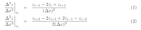
6. **Estimates the numerical error in the calculations of Requirement 4. Perform this using numerical derivatives for as many data points as possible; at the ends of the data, use the value closest to the end (e.g. for the 1st datum, use the second derivative calculated at the 2nd datum, and the third derivative calculated at the 3rd datum).  For data spaced evenly in x, the necessary formulae are [the methods are O(∆x2) accurate]:

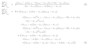
For data unevenly  spaced in x, the necessary formulae are [the methods are O(∆x) accu- rate]:

7. Plots the results from Requirements 4 and 6. Also plots ∂z/∂x (correct Requirement 4 us- ing Requirement 6) together with the central difference from Requirement 4. On the plots of the gradient, also show the viaduct average gradient. Discusses the results, including which is the best method.

8. Has appropriate comments throughout.

1.3    Assessment Criteria

Your code will be assessed using  the following scheme. Note that you are marked based on how well you perform for each category,  so the correct answer determined in a basic way will receive half marks and the correct answer determined using an excellent method/code will receive full marks.

Quality of hand calculations	30 marks
Quality of difference calculations	30 marks
Quality of verification	5 marks
Quality of error calculations	30 marks
Quality of the plots	10 marks
Quality of the discussion	5 marks
Quality of header(s) and comments	5 marks

Q 2     (worth 90 marks)

2.1      Introduction

The resistance of a resistor which has a constant cross-sectional area A can be calculated using the formula

R=ρL/A ,                                        (5)

where ρ is the resistivity and L is the length of the resistor. If the geometric and/or material properties are not constant, then (because each x-location can be considered to be a resistor in series) the formula is:

R=∫L ρ(x)/ A(x) dx                (6)

Thermoelectricity is a phenomenon that  relies on changing material properties:  electric currents produced by an applied voltage difference generate heat (which could replace chemical means), or temperature differences generate potential differences (most commonly applied in thermocouples). It is, however a very inefficient means of converting between heat and electricity (especially compared to heat engines using chemical reactions to drive an electric generator), which is fundamentally due to the relevant material properties.

For your assignment, the following values are to be used for resistivities, radii and lengths. The properties for resistor 1 are:

ρ1    =  1.68 × 10−8  Ωm

r1     =   1 mm

L1     =  1 cm ,

 resistor 2:

ρ2    =  (1 + 0.95179 × 10) × 10−8  Ωm

r2     =   1 + 8.8395 ÷ 10 mm

L2      =  1 + 6.9848 ÷ 10 cm ,

 and resistor 3:

ρ3    =  (1 + 9.198 × 10) × 10−8  Ωm

r3     =   1 + 7.2579 ÷ 10 mm

L3      =  1 + 2.0632 ÷ 10 cm .

In this question, you will calculate the resistances of a number of different resistor configu- rations:

1. Resistor 1 with uniform cross-section.

2. Resistor 1 with radius r1 at the start and radius 2r1at the end (the radius changes at a constant rate between the two ends).

3. A resistor constructed by joining resistor 2 end-to-end with resistor 3 (the component resistors each have a constant cross-section).

4. *A resistor constructed by joining resistor 2 end-to-end with resistor 3 (the radius changes at a constant rate along each of the two component resistors so that the radius is r1 where they join).

2.2    Requirements

For this assessment item, you must perform hand calculations:

1. Find the resistances of configurations 1–4 analytically.

2. Use the trapezoidal method to determine the resistance of configurations 2 and 3 using four intervals along the total length of each configuration.  Validate the results with Requirement 1.

You must also produce MATLAB code which:

3. Repeats Requirement 2 and verifies the code.

4. Uses the trapezoidal method to solve configurations 1–4 using appropriate intervals.

5. Reports the values from Requirements 1 and 4.

6. *Estimates, reports and discusses the overall numerical error in the calculations of each configuration in Requirement 4.

7. Plots R(x) from Requirements 1 and 4.

8. Has appropriate comments throughout.

2.3    Assessment Criteria

Your code will be assessed using  the following scheme. Note that you are marked based on how well you perform for each category,  so the correct answer determined in a basic way will receive half marks and the correct answer determined using an excellent method/code will receive full marks.

Quality of hand calculations	30 marks
Quality of trapezoidal calculations and discussion	35 marks
Quality of error calculations	10 marks
Quality of the plots	10 marks
Quality of header(s) and comments	5 marks

3    (worth 145 marks)

3.1    Introduction

We return to Assignment 1. Your task is to simulate the droplet acceleration using the formulae and parameters supplied in Assignment 1, and starting with the initial  condition supplied in ass1in.csv.

To obtain consistent results from your random number generation, you should initialise the seed to a fixed value using rng(seed).  For your assignment, the value is:

seed = 8.2756

 3.2    Requirements

For this assessment item, you must perform hand calculations:

1. Use Euler’s method to estimate the velocity for the 2nd data value in ass1in.csv using 5 equal steps; validate against that data value.

You must also produce MATLAB code which:

2. Repeats Requirement 1 to verify the method.

3. Simulates the entire duration of ass1in.csv using appropriate parameters for the following methods:

(a) Euler’s method

(b)  ode23 (c) ode45

Reports the timestep used for Euler’s method; if you use the default settings for the MATLAB ode solvers, report this, otherwise report what values you used for any changed settings.  Graphically validates the simulation results with  the data in ass1in.csv and reports the outcome of the validation.

4. Uses Simulink to:

(a) Simulate up to the 5th data value.

(b)  ***Simulate the entire duration of ass1in.csv.

Plots the results and reports the final velocity within Simulink. Uses MATLAB to validate the results with the data in ass1in.csv.

5. ***Simulates droplet collisions and accelerations.

(a) Loads the data in ass2in.csv and multiplies the velocities by 50.

(b)  Assigns each droplet an “age”. The age grows  so that, on average, for each 0.5 mm the droplet travels, it collides with another droplet. Initialise the age of each droplet to be a uniformly-distributed random number between 0 mm and 1 mm.

(c) At each timestep, accelerates every droplet according to Euler’s method as in Re- quirement 3.

(d)  For each  timestep, increments every droplet’s age.  If  the age is greater than a uniformly-distributed  random number between 0 and 1 mm, then the droplet is to collide after the new velocity has been calculated  for the timestep.

(e) Pairs up droplets that are to collide and collide them according to the algorithm of Assignment 2. Randomly assign droplets to be paired with each other.  If there is an odd number of droplets marked for collision, choose one to not collide. Reset the age of the new, combined droplet according to the initialisation in Requirement 5b.

(f ) Simulates up to the entire duration of ass1in.csv.

(g) Plots the mean velocity, standard deviation of velocity and total number of droplets as functions of time.

(h)  Reports to the Command Window the total number of droplets remaining at the end of the simulation. If there is only a single droplet remaining, reports when the last droplet collision occurred.

6. Has appropriate comments throughout.

3.3    Assessment Criteria

Your code will be assessed using  the following scheme. Note that you are marked based on how well you perform for each category,  so the correct answer determined in a basic way will receive half marks and the correct answer determined using an excellent method/code will receive full marks.

Quality of hand calculations	30 marks
Quality of Requirement 2	20 marks
Quality of Requirement 3	30 marks
Quality of using Simulink	30 marks
Quality of simulating droplet collisions and acceleration	15 marks
Quality of the plots	15 marks
Quality of header(s) and comments	5 marks