Looking for Standard Costs and Variances Analysis Question to answers solution? Gets Cost Accounting Assignment Help, Accounting Case Study Solution & MBA Essays Writing from PhD/MBA Accounting experts at cost-effective rates? Acquire HD Quality research work with 100% Plagiarism free content – Get related Finance Assignment Help & Topics written by native Expert writers in USA, U.K. & Australia.

Standard Costs and Variances Analysis Questions to Answers

A standard cost is a measure of how much one unit of product or services should cost to produce or deliver. With such a reference point established, the actual cost to produce or deliver a unit can be evaluated. Variances of actual cost from standard cost can be evaluated, and reasons for variances may suggest corrective action or highlight the need to consider changing the standard cost. Standard cost accounting systems are usually less costly to use because they require less record keeping. Once a standard cost is established, it provides a basis for decisions, a basis for analyzing and controlling costs, and a basis for measuring inventory accounts and cost of goods sold.

Standard costs may be established using careful analysis of the product or service and the materials and process used to create it. Standard costs established in this way could be thought of as ideal costs, and actual costs may differ from such costs because of actual price differences, errors or mistakes, or changed conditions from the ideal. However, other ways of determining standard costs are also common. For example, actual cost this year can be compared to the “standard” established by spending and performance in a prior period, such as when we compare cost this year to cost last year. Because standard costs are only reference points, measurements to anchor analyses and the questions they raise, there is nothing inherently good about favorable variances or bad about unfavorable variances from standard costs.

Although the remainder of this note emphasizes manufacturing cost variances, many of the same concepts can be applied to the delivery of services. The focus on manufacturing allows a more orderly discussion of material and overhead variances, which are often harder to conceptualize in service organizations.

Prime Cost Variances

The term prime costs refers to the material and labor costs that can be directly related to a unit of product. The standard for any element of prime cost involves two components: a price component and a quantity component. The standard cost is the standard quantity to be used multiplied by the standard price per unit of measure. For example, if an electric motor contains four bushings and each bushing should cost $.25, then the standard cost for bushings is $1.00 (standard quantity of 4 ´ the price per unit of $.25). Variances are usually computed for each of the two components for both material and labor costs. The formulas for calculating the variances are as follows:

Price variance (PV) = (SP – AP) x AQ

Quantity variance (QV) = (SQ – AQ) x SP

Total variance (TV) = PV + QV

or

Total variance (TV) = (SP x SQ) – (AP x AQ)

where

SP = standard price

AP = actual price

SQ = standard quantity

AQ = actual quantity

Since the total variance is the difference between the standard cost allowance (SP ´ SQ) and the actual cost incurred (AP ´ AQ), you should be able to verify for yourself that the price and quantity variance in the above formulas do sum to the total variance.

An example of the calculation of prime cost variances is shown in Exhibit 1.

Some Complications

You may have wondered why the quantity variance is computed using standard prices, whereas the price variance is computed using actual quantities. Most people feel that price fluctuations should not be considered when measuring the variance due to quantity fluctuations— vary only one component at a time. However, most people also feel that the price variance should be measured over the actual quantities for which the price difference obtains, not the standard quantities. Some people do not like this logical inconsistency. They prefer to vary only one component at a time in both the price and quantity variance calculations. They then set up a third variance (joint variance) caused by the joint fluctuation in both prices and quantities. Under this approach the formulas are as follows:

PV = (SP – AP) x SQ

QV = (SQ – AQ) x SP

JV = (SP – AP) x (AQ – SQ)

TV = PV + QV + JV

This can be illustrated graphically as follows, assuming both price and quantity variations are unfavorable:

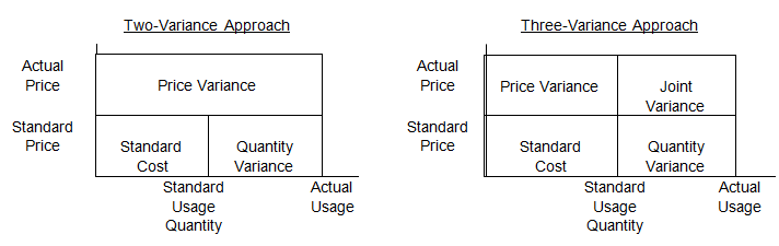
It is difficult, if not impossible, to give a common-sense interpretation to the joint variance when one of the two components varies favorably and the other varies unfavorably. Furthermore, we believe that purchasing agents should be assessed for price variations on quantities actually purchased, but that production managers should be assessed for quantity difference times standard prices, ignoring price fluctuations. For these reasons, we favor the simpler, two-variance approach.

The logically consistent framework we have set up in this note that PV + QV = TV is often violated in practice in regard to material variances. Many firms prefer to compute the price variance over quantities purchased and the quantity variance over quantities used. Since purchase and usage quantities often differ in any given period, the two variances cannot be summed algebraically. They can, however, still be combined for cost reporting purposes to get a picture of purchasing and usage variances together.

Suppose, for example, that in the example in Exhibit 1, material purchases totaled 30 pounds at $.80, even though only 25 pounds were used in production. The material variance calculations could then be as follows:

Price variance: ($1.00 – $.80) x 30 lb = $6 Favorable

Quantity variance: (20 – 25) x $1.00 / lb = $5 Unfavorable

Total variance: $6F + $5U = $1F ¹ $20 – $20

A labor price variance is often called a labor rate variance, and a labor quantity variance is often called a labor efficiency variance. A material quantity variance is often called a material usage variance, and a material price variance is often called a purchase price variance.

Overhead Cost Variances

Budgets for prime costs hinge on unit-level standard costs. Once standard prime costs per unit are determined, the budget for any given period is just the standard per unit times the number of units produced. A simple approach like this works because prime costs are variable costs. The cost allowance or budget thus varies directly as production volume varies. Because manufacturing overhead costs do not all vary directly with volume, it is a more difficult task to determine allowable overhead at any given level of production.

Overhead Budgets

One approach to overhead budgeting ignores the volume dependence issue entirely. This approach is called fixed overhead budgeting. Under a fixed-budget approach, management determines the amount of overhead that should be incurred at the normal or most likely production level. This expense total becomes the budget against which cost performance is measured regardless of the level of production output actually achieved. To the extent that manufacturing overhead costs vary with production, the fixed-budget approach yields less and less meaningful variance data, the more that actual output varies from planned or normal output. There is no conceptual support for a fixed-budget approach to manufacturing overhead. We would not bother to mention this approach except that some organizations still use it.

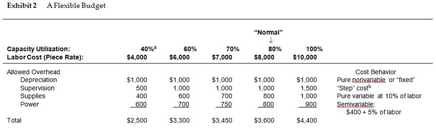
The more conceptually sound approach to determining overhead standards is called flexible budgeting. A flexible overhead budget specifies allowable cost at each possible output level. Once a period is completed and the actual production volume is known, the budget standard is determined by reference to the flexible budget for the level of output. This is a direct parallel to the way a budget for direct material and direct labor is determined. If all overhead is assumed to be either pure “variable” or pure “fixed,” a flexible budget is just a formula of the following type:

Budget allowance = a + bx

where

a = fixed overhead costs for the period

b = variable overhead costs per unit

x = units produced during the period

Overhead cost behavior is not this simplistic and is not assumed to be in most businesses today.

An example of a more complicated but still simplified flexible budget is shown in Exhibit 2.

Overhead Absorption

Because manufacturing overhead costs are considered to be product costs, it is necessary to find some way of charging or absorbing them into inventory. However, the simple approach of charging actual manufacturing overhead directly to work-in-process (WIP) inventory is usually not considered to be an acceptable approach, for two reasons:

1. Overhead variances are not usually considered to be product costs. Variances do not add value to the inventory. Thus, only allowable overhead is to be inventoried.

2. Volume considerations also affect the decision of how much overhead to absorb in inventory. Suppose, for example, depreciation is $1,000 per period and that 1 unit is produced in period 1 and 1,000 units are produced in period 2. It doesn’t seem “fair” to most accountants to say that a period 1 unit carries a cost of $1,000 for depreciation (1 unit /$1,000 depreciation) and a period 2 unit only $1 (1,000 units / $1,000 depreciation). A unit cannot really be “more valuable” just because fewer were produced that month. “Fair” allocation of depreciation to inventory seems to require a concept of normal volume. The $1,000 depreciation expense is incurred as a “reasonable” charge on the assumption that some reasonable or normal number of units will be produced on the equipment. It is this normal volume level over which the planned overhead should be spread, so the argument

For these two reasons, standard practice for charging manufacturing overhead into inventory is to set an absorption rate computed as planned overhead costs at normal production volume (per the flexible budget) divided by that normal volume. In the example shown in Exhibit 2, the normal volume is 8,000 direct labor dollars (80% of capacity). At this level of output, budgeted overhead is

$3,600. The overhead absorption rate is thus $3,600 /$8,000, or $ .45 per direct labor dollar. In single- product firms, output can be expressed in units of product. In multiproduct firms, however, it is necessary to set some other measure of capacity utilization, such as labor hours, labor dollars, or machine hours. The choice of a volume measure in a particular business should be based on which variable best measures the level of capacity utilization for that business.

The accounting works as follows: A T-account is established in the books of account called factory overhead, or burden, or something equivalent. Actual manufacturing overhead expenses are charged (debited) to this T-account. Overhead is absorbed into inventory by crediting the factory overhead account and debiting the WIP inventory. The amount of absorbed overhead is equal to the absorption rate times the actual volume attained. In the example in Exhibit 2, if actual volume was 7,000 direct labor dollars, $3,150 of overhead would be charged to WIP ($7,000 x $ .45).

You will note that this absorption process will only “clear” the factory overhead account if two conditions are both met:

1. If actual volume equals normal or planned volume. Manufacturing overhead does not vary directly with production. The absorption rate, however, is a pure variable rate. Thus, absorbed overhead will only equal planned overhead at one particular volume level—that level used in computing the absorption rate.
2. If actual overhead expenses equal planned expenses per the flexible budget. Since only budgeted overhead is absorbed, any differences between budgeted costs and actual costs will not be “cleared” from the factory overhead T-account.

At the end of any accounting period, therefore, any residual balance in the factory overhead account results from failure to meet one or both of these two conditions. This end-of-period residual in the factory overhead T-account is sometimes called the book overhead variance because it is what shows up in the books of account. It is also sometimes called the total overhead variance.

Normal accounting practice is to charge this variance to cost of goods sold for the month as a period expense, rather than to try to add it to product costs.

Analyzing the Total Overhead Variance

For purposes of evaluating cost-control performance, the relevant comparison is actual overhead versus allowed overhead per the flexible budget. Assuming actual overhead expenses as follows, this calculation for the example in Exhibit 2 would be:

Cost Item	Flexible Budget Allowance at Actual Volume of 7,000 Direct Labor Dollars	Actual Expense at Actual Volume	Spending Variance
Depreciation	$1,000	$1,100	$100U
Supervision	1,000	1,050	50U
Supplies	700	690	10F
Power	750	770	20U
Total	$3,450	$3,610	$160U

The difference between actual overhead incurred and the flexible budget at this level of output is called the overhead spending variance. It measures cost control performance.

 

You will remember that the total variance which shows up in the T-account is equal to the difference between actual overhead (the debits) and absorbed overhead at actual volume (the credit). The variance that is useful in measuring cost-control effectiveness (the spending variance) is equal to the difference between actual overhead and allowed overhead at actual volume. In order to present an analysis that explains the total overhead variance, cost accountants need to have some name for the difference between the total variance (actual OH1—absorbed OH) and the spending variance (actual OH—allowed OH). Using a little algebra, you can see that the quantity for which we need a name is allowed OH—absorbed OH. Then, this quantity plus the spending variance equals the total variance:

(Actual OH – allowed OH) + (allowed OH – absorbed OH) = (actual OH – absorbed OH) Spending variance   + “plug” = total variance

Regarding the plug, we have already observed that allowed OH will only equal absorbed OH when the firm operates at normal volume. Why? Because budgeted overhead does not vary directly as production varies, but absorbed overhead is purely variable, by convention. The absorption rate is set to just absorb into inventory the planned overhead when the firm actually operates at its normal volume. Standard (absorbed) overhead cost per unit, for purposes of valuing inventories, is thus equal to a proportional share of budgeted overhead when production volume is at normal levels.

This means that the difference between allowed OH and absorbed OH relates to the difference between normal production volume and actual production volume.

Because the plug variance (allowed OH — absorbed OH) results from the difference between planned and actual production volume, it is called a production volume variance. The dollar amount of this production volume variance has no particular management significance whatsoever. The dollar amount is just the plug required to reconcile a managerially significant number (the spending variance) to a number that shows up in the income statement (the total variance). The production volume variance does result from variation between planned and actual production volume. In this sense, the name is appropriate.  However, the amount is not managerially useful—the amount is just a plug. For our example in Exhibit 2, the amount is computed as follows:

Total variance = actual OH – absorbed OH = $3,610 – $3,150 = $460 Unfavorable

Spending variance = actual OH – allowed OH = $3,610 – $3,450 = $160 Unfavorable

Production volume variance = total variance – spending variance = $460U – $160U = $300U

or

Production volume variance = allowed OH – absorbed OH = $3,450 – $3,150 = $300U

Going one step further, we can talk about what comprises the plug. In a nutshell, it is made up of under- or over-absorbed fixed manufacturing overhead. It does not include any variable overhead because items that are directly variable with production are treated identically in the absorption rate and in the flexible budget. They thus cancel out in computing the difference between allowed and absorbed cost. In our illustration, for example, the absorption rate of $ .45 per direct labor dollar includes $ .15 of variable cost, and the flexible budget also includes $ .15 per direct labor dollar of variable cost ($ .10 for supplies and $ .05 for power). At actual volume of $7,000 direct labor dollars, therefore, the allowed OH of $3,450 includes $1,050 of variable cost, and the absorbed OH of $3,150 also includes $1,050 of, variable cost. This $1,050 thus does not contribute anything to the difference between $3,450 and $3,150. The difference is the fixed-cost absorption rate ($ .30) times the unfavorable volume fluctuation of $1,000 direct labor dollars, or $300 Unfavorable. The $ .30 fixed- cost absorption rate is equal to the $2,400 of planned fixed overhead at normal volume divided by the volume measure of 8,000 direct labor dollars. The overall absorption rate of $.45 is just the sum of the variable part and the nonvariable part.

Conclusion

The important questions that follow the calculation of variances concern why actual costs were different from standard costs. Sometimes the answers are obvious, but often they are not. For example, material that cost less than standard may have been of lower quality than expected, causing more material to be used and requiring more labor time to be spent by workers of high skill (and higher wage rates). Or maybe production delays reduced the quantity produced below planned volume. Skilled managers analyzing variances often try to weave clues together into a “story” that explains what is going on so that they can think about what to do differently in the future.

Total variance (actual OH – absorbed OH): $3,610 – $3,150 = $460 Unfavorable

Spending variance (actual OH – allowed OH): $3,610 – $3,450 = $160 Unfavorable

Production volume variance (total variance – spending variance): $460U – $160U = $300U

or

Production volume variance (allowed OH – absorbed OH): $3,450 – $3,150 = $300U

Exhibit 1      Calculation of Prime Cost Variances

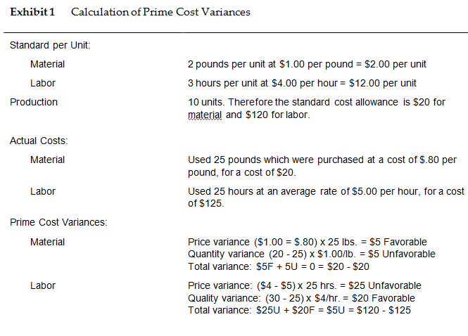
Exhibit 2  A Flexible Budget