1.  (Worth 100 marks)

Introduction

To do something useful with big data, models are devised from the large numbers of observations in order to predict what will occur for some other observation(s). A simple linear model¹ is of the form:

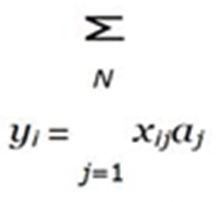
where y_i is the dependent variable, i is the observation number (there are a total of M observa- tions), x_ij is the set of independent variables, N is the number of independent variables (for big data, M N ), and a_j are the set of model coefficients. Equation (1) lends itself to a matrix formulation:

Y = XA

The  model  coefficients  a_j  are  determined  by  measuring  y_i  and  x_ij.   One of  the  dangers of developing such a model is “over-fitting” the data. This is where a_j are tuned for the M observations so that a_j is an excellent model for y_i, i ≤ M , but is a poor model for y_i, i > M .  Good practice is therefore to split the M observations into a “training dataset” (with M₁ observations,  M₁ ≥ N  and  typically  M₁    N ) and  a  “test  dataset”  (with  M₂ observations, M₁ + M₂ = M , and typically M₂ < M₁). The  values  of  a_j are  determined  from  Eq.  (1)  using the training dataset (with M₁ observations). The values can then be validated using the test dataset by calculating y_i using Eq. (1) and calculating the error from the actual values yˆ_i.

In this question, you are going to apply this methodology to determine if it is possible to estimate the mean pressure for the year based on temperature readings from each month. The ideal gas law is:

p = ρRT

where p is the pressure, ρ is the density, R the ideal gas constant and T the temperature.

Your computational task is to use Eq. (1)

in the form of Eq. (2)

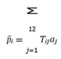
P = TA

for  the  9:00  readings.   Here  p¯_i is  the  average  pressure  across  all  months  for  day  i,  T_ij is  the temperature on day i and month j  and a_j is the average coefficient for month j.  You  will use  the entire 12 months’ worth of data (N  = 12) to calculate the average pressure for each calendar  date (M  = 28 since there are only 28 days in February), i.e. p¯₁ is the average pressure calculated using the 1st of July, 1st of August, 1st of September, etc. For your assignment, the following value is to be used:

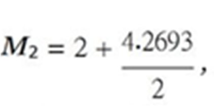
where M₂ is to be rounded to the nearest integer. Because M > N (we don’t have M N ), we will work with M₂ ≤ N , which is not ideal, but is pragmatic, since it guarantees that M₁ > N   to produce statistically-good estimates of a_j.

Requirements

For this assessment item, you must perform hand calculations using Eq. (5):

1. Calculate a₁ using only the 1st of July (i.e. M = 1, N = 1).
2. Calculate a₁ and a₂ using only the 1st and 2nd of both July and August (i.e. M = 2, N = 2).

You must also produce MATLAB code which uses Eq. (5):

1. Repeats Requirements 1 and 2. Reports and verifies the
2. *Successfully loads all the relevant
3. *Repeats Requirement 2 using the loaded data. Reports and verifies the
4. **Reports the value of M₂ before it is rounded, to confirm the values of M₁ and M₂ you are to use. Calculates all the a_j using the training dataset of M₁ values and reports a_j.
5. **Uses the test dataset of M₂ values to assess the quality of the modeled values of p¯_j.
6. ***The accuracy of the results is limited because the variability in the temperature  and pressure data is  in  the  3rd  or  4th  significant  figure,  and  also  because  we  do  not  have big data. To remedy  the  problem  of  significant  figures,  the  data  should  be  The first normalization technique to use in this circumstance is to “centre” the data in        the matrix T (subtract a constant  value,  sometimes  the  mean,  from  all  the  data),  which  will make the variability in the 1st or 2nd significant figure. Use 15^◦C to centre  the  temperature data, produce  new  a_j  from  your  training  dataset  and  test  the  coefficients.  See if you achieve some further numerical improvement in this case by  “scaling” the data   in T (non-dimensional sing, normally  by dividing  by  the  standard  deviation)  so  that  all  the quantities are of the same order of magnitude².
7. Discusses the
8. Have appropriate comments

The projected difficulty of a Requirement is indicated by the number of * at the start. All students are expected to be able to complete Requirements which do not have an *.

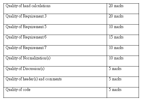
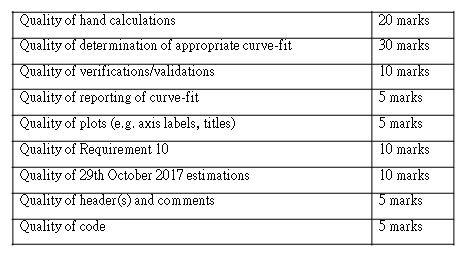
Assessment Criteria

Your code will be assessed using the following scheme. Note that you are marked based on how well you perform for each category, so the correct answer determined in a basic way will receive half marks and the correct answer determined using an excellent method/code will receive full marks.

2.  (Worth 100 marks)

Introduction

When data is being measured, it is common for there to be data missing, which could be due to a fault in the measuring equipment, or the variable being unmeasurable at that moment. In the weather data for Dalby, the maximum temperature was not recorded on 29th October 2017, presumably because not all the temperature readings were recorded for that day, so therefore it is impossible to know whether the highest recorded temperature was actually the maximum. Leaving unknown/unreliable readings blank is the best option, since inserting a value (such as zero) could be a valid value, and therefore pollutes the data (this is why my preferred option is to fill an empty slot in an array with NaN, since it is unlikely to have occurred from a calculation). If you need to be able to use a value where there is one missing, then you need to use some method of including an intelligent guess. In this question, you will use a global curve-fit to provide the guess. All of you will use T₃ (the temperature measured at 3:00 pm) as the independent variable to model the maximum daily temperature, T_max. You will also compare the outcome for this modelling to using another variable, V , as the independent variable. For Your assignment, the following value is to be used:

Q₂ = 4.1501 .

The independent variable (besides T₃) you are to use is based on your value of Q₂:

V ≡ T_min ,  Q₂ ≤ 5

V  ≡ T₉ ,       Q₂ > 5

where T is temperature and the subscript refers to either the daily minimum or the particular time of day.

Your  task is to estimate the value  of T_max on 29th October 2017 using both T₃ and V as   the independent variable.

Requirements

For this assessment item, you must perform hand calculations using T_max and T₃:

1. Take the values from 28th and 30th October 2017 and estimate the coefficients of the three standard curve-fitting functions. These data points will provide a qualitative repre- sensation of the overall

You must also produce MATLAB code which:

2. Repeats Requirement 1 and verifies the
3. *Performs curve-fits of all the data for T_max and T₃. Use the MATLAB function isfinite to filter the dataset so that only those dates with recordings of both T_max and T₃ are included.
4. Validates the three standard curve-fitting functions obtained in Requirement 3  by  com-  paring with the parameters obtained in Requirement 1. Given the limited data used in Requirement 1 and the overall scatter in data, don’t expect the values to be very
5. Determines which curve-fit is the
6. Demonstrates that the chosen curve-fit is the best both graphically and numerically, show- ing both the data and the relevant curve-fit.

7. Displays a message in the Command Window stating which type of curve-fit was chosen, stating the parameters of the curve-fit and the result of the numerical test of the curve-fit.
8. Plots the best curve-fit along with the data in a separate figure with normal-scale
9. Uses the best curve-fit to estimate T_max for 29th October
10. *Reports the value of Q₂, leading to the selection of V . Repeats Requirements 3, 8 and 9 using only a linear curve-fit with V the independent variable instead of T₃. Plots the curve-fit along with the Compares and discusses the two estimates for T_max.
11. Have appropriate comments

The projected difficulty of a Requirement is indicated by the number of * at the start. All students are expected to be able to complete Requirements which do not have an *.

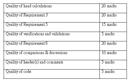
Assessment Criteria

Your code will be assessed using the following scheme. Note that you are marked based on how well you perform for each category, so the correct answer determined in a basic way will receive half marks and the correct answer determined using an excellent method/code will receive full marks.

3  (Worth 100 marks)

Introduction

This question provides an alternative methodology to the problem in Question 2. In this question, you will use interpolation to provide the guess. Time is an obvious independent variable to use, but Question 2 suggests that there are other options. For your assignment, the following value is to be used:

Q₃ = 2.4937 .

The independent variable (besides time), V , you are to use is based on your value of Q₃:

V ≡ T_min ,  Q₃ ≤ 5

V  ≡ T₃ ,       Q₃ > 5

Where T is temperature and the subscript refers to either the daily minimum or the particular time of day.

Your task is to estimate the value of T_max on 29th October 2017 using these two independent variables. For this problem you are to only use data from 19th to 31st October inclusive (a total of 12 days not including 29th October). These dates have been chosen to ensure that you do not have repeated values of the independent variable (which is numerically problematic) and also that you have sufficient data either side of 29th October for the interpolation methods to be numerically reliable.

Requirements

For this assessment item, you must perform hand calculations:

1. Estimate the maximum temperature on 29th October 2017 using linear interpolation with time the independent
2. **Repeat Requirement 1 using V as the independent variable. You must also produce MATLAB code which:
3. Repeats Requirements 1, reporting the result to the Command
4. Verifies Requirement
5. Repeats Requirement 1 using cubic splines. Additionally validates the result with Re- quirement
6. ***Reports the value of Q₃, leading to the selection of V . Repeats the calculations of Requirements 3–5 using V as the independent variable. The results using the cubic spline method will not be very good for one reason or another. The function sortrows
7. Compares and discusses the 2 answers for T_max on 29th October 2017 from Question 2 and the 4 answers from this
8. Has an appropriate comment

Assessment Criteria

Your code will be assessed using the following scheme. Note that you are marked based on how well you perform for each category, so the correct answer determined in a basic way will receive half marks and the correct answer determined using an excellent method/code will receive full marks.

4.  (Worth 100 marks)

Introduction

Predicting what will occur is the essence of a model. Many people rely on weather forecasting for their livelihood, and many more people for their ordinary lives. Your task is to devise and construct a simple model for two of the variables in the Bureau of Meteorology dataset: the temperature at 3:00 pm (T₃) and the relative humidity at 9:00 am (φ₉).

To obtain consistent results from your random number generation, you should initialise the seed to a fixed value using rng(seed). For your assignment, the value is:

seed = 1.1259

Requirements

For this assessment item, you must perform hand calculations on the data for July:

1. Calculate the sample mean and standard deviation for T₃ and φ₉ for the first 10 data values of each
2. Use the first 20 data values T₃ and φ₉ to estimate the sample pdf (i.e. the scaled frequency). Plot the sample pdfs. You can produce the plots in MATLAB, but you must perform the calculations of the value of the pdf for each value of T₃ or φ₉ by

You must also produce MATLAB code which:

3. Repeats the hand calculations and verifies the MATLAB
4. Loads the entire 12 months’ worth of data. The rest of the analysis is to be on the full dataset in this file³.
5. *One of T₃ and φ₉ can be represented by a standard distribution. Determine which variable and the corresponding distribution which best describes the variable, including proof that this distribution is an appropriate model and proof that the other variable cannot be modelled by the same distribution. Part of this proof may be demonstrated by completing Requirements 6–8.
6. *Calculates the parameters of the population distribution for both variables, including the associated error in the estimation of the parameters. Reports the values to the Command Window.
7. *Calculates the sample mean and sample standard deviation for both variables, along with an assessment of the accuracy of these
8. *Graphically compares the sample pdf and population pdf for both
9. *Reports to the Command Window a discussion of the applicability of the population distribution for both
10. **Performs modelling for only the chosen variable from Requirement 5. Produces a prediction of the values for the 12 months by randomly generating samples from the distribution. Plots the time series of values which is thus produced along with the history of the recorded values. Discusses the validity of the predicted values in predicting the actual history (some analysis will assist you in drawing conclusions).
11. Has an appropriate comment

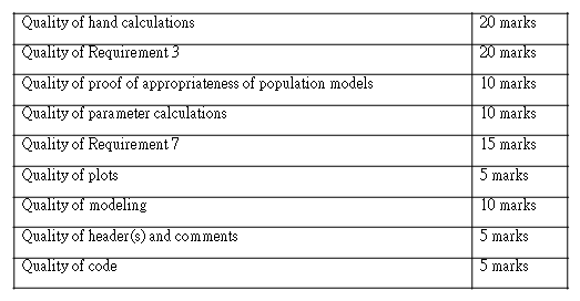
Assessment Criteria

Your code will be assessed using the following scheme. Note that you are marked based on how well you perform for each category, so the correct answer determined in a basic way will receive half marks and the correct answer determined using an excellent method/code will receive full marks.

Submission

Submit your code, with the *.csv files that are provided to you, by the due date to the Study- Desk. Submit your hand calculations as a pdf file. Note that:

• You do not need to rename your files when uploading: the system automatically segregates different students’
• If you can see that the files have uploaded, then you have successfully submitted your assignment. There is no need to click a “send for marking” button, but you will have to click a button confirming that the submission is your own
• You MUST upload all of your code along with input/output files in a *.zip file. The following are the only file types that can be submitted:
  • *.zip
  • *.pdf
  • *.doc
  • *.docx

The system will block any attempt by you to upload a file which doesn’t match any of those file extensions.

• If you forgot to submit a file, do not upload it after the due date:  the submission time       is based on when the last file was You should email the examiner in this circumstance (with any file attached). If you remember close to midnight on the day you made your submission, you only need to upload the file (don’t bother emailing), since the submission day will effectively be the same.