BILIRUBIN – Chemistry QA/QC Assessment Analysis

 

Assignment Details:-

• Topic: Chemistry QA/QC
• Document Type: Essay (any type)
• Subject: Chemistry
• Number of Words: 1000
• Citation/Referencing Style: Harvard

 

 

Abstract

This report assesses the performance of the Konelab Automated Analyser to determine the concentration of total bilirubin.

Using what type of assay. How it is measured. Standard curve. Causes for results. What the results indicate/ clinical significance. Finally, the report concludes with a brief discussion of possible treatments and consequences of results. Quality control data from total bilirubin assays were recorded onto a Levy-Jennings chart for quality control purposes. The total bilirubin data set was determined to be non-Gaussian and therefore non-parametric statistics had to be used to determine reference intervals. Alternatively, the total bilirubin data set was determined to be normally distributed, resulting in the generation of reference intervals from parametric statistics i.e. from 95% of the population. It was concluded that the XXX Assay consistently estimated a higher SERUM/PLASMA TOTAL BILIRUBIN concentration than did the XX method (Table x); a discrepancy that is possibly the result of using 2 different types of methods.

 

Introduction

Bilirubin exists in two forms: unconjugated (indirect) bilirubin and conjugated (direct) (1). In plasma, unconjugated bilirubin is bound and transported by albumin to the liver (2). Bilirubin after conjugation is water soluble and primarily excreted into bile and small intestine (2). The normal level of serum bilirubin is less than 1mg/dL (20 mol/L) (1). Hyperbilirubinaemia is caused by either excessive formation of bilirubin or inadequate removal of bilirubin in the bile, resulting in a yellowing of the skin, also known as jaundice (3). The elevation of bilirubin production may result from the increased breakdown of haemoglobin of erythrocytes in haemolysis (4). Alternatively, disorders of impaired conjugation of bilirubin are caused by inherited aetiology, such as Gilbert’s syndrome, Crigler-Najjar syndrome or liver diseases due to drugs, alcohol, biliary obstruction due to gallstone, cholangitis (2, 3).

Serum bilirubin can be measured by several methods, including spectrophotometric, chromatographic, and capillary electrophoretic methods (3). The most frequently used methods is based on diazo coupling reaction, which measures the total bilirubin and direct bilirubin (3). In this project, total bilirubin is measured by an automated analyser Konelab 20XT, based on diazo coupling method. A series of experiments were conducted, including setting up a Quality Assurance Program (QAP), comparison of two methods from two different laboratories, determination a reference interval for a specific population, interference study, and linearity study.

 

Materials

• Konelab Analyser 20XT and associated equipment
• 5mL rubber bulb pipette
• 2mL skirted micro-test tubes
• 10mL plastic test tubes, fit for Konelab segment
• Rocker, roller or similar mixing apparatus
• Thermoscientific Total Bilirubin Reagent A (NBD) – LOT: S678.
• Thermoscientific Total Bilirubin Reagent B (NBD) – LOT: S732
• Lyphochek® Assayed Chemistry Control 1 – LOT: 26461
• Lyphochek® Assayed Chemistry Control 2 – LOT: 26462
• Calibrator for Automated Systems (C.f.a.s.) – LOT: 32411701
• Distilled water
• General laboratory equipment

 

 Method

1. In order to measure the concentration of Bilirubin, Konelab Analyser was configured according to the parameters described ‘Total Bilirubin – NATA’.
2. Reconstitute control 1, control 2 and the calibrator by pipetting 5mL and 3mL of distilled water into each system respectively before mixing thoroughly or leaving on a rocker, roller or similar mixing apparatus until homogenous. Allow the calibrator to stand at room temperature for at least 20 minutes after reconstitution before assaying.
3. Pipette approximately 2mL of each control 1, control 2, calibrator and distilled water (as singlets) into separate, appropriately labelled 2mL skirted micro-test tubes. Insert those microtubes (without their lids) into larger plastic test tubes ready for insertion into the Konelab when prompted.
4. After removing their lids, insert reagent bottles A and B into the Konelab machine when prompted, ensuring that there are no bubbles on the surface of the bottle. Insert the loaded segment containing and the blank, calibrator, and controls 1 and 2 into the Konelab when prompted.
5. Run the calibration and control check for the assay parameters input earlier. A calibration curve is generated from the measured calibration concentrations. Calibration and control values need to be accepted manually and will need to be repeated if unacceptable.
6. When prompted, load each of the 30 patient samples into a separate 2ml cuvette contained within a segment, taking note of the barcodes assigned to each tube.
7. The Konelab system will analyse the data and accept results automatically if they are within the predetermined control limits. The raw absorbance data used to calculate the bilirubin concentrations can be exported along with sample size, mean, standard deviation, and a coefficient of variation (%CV) of the duplicated controls and sample data.

 

The results were then plotted on Levy Jennings chart (Appendix) for visual examination of controls’ values based on Westgard rules. After 14 times of repeated measurement, QC range, Standard deviation (SD) and Coefficient of variation (%CV) for each control were established.

 

In addition, in order to examine the precision and accuracy of the method, 16 patients’ samples with known value of total bilirubin were assayed in the second exercise. The obtained results were plotted against the target values. The total error (TE) is the combination of the systematic error (SE), which was calculated from the Linear regression, and the random error (RE), which was calculated from SD of the QC at each decision level of bilirubin. The total error is then compared to the allowable error value at each decision.

 

In the exercise of comparison two methods, total bilirubin concentration of 30 patients were measured by UTAS and Launceston General Hospital (LGH) laboratories. Two groups of bilirubin results were analysed by using Deming regression. The difference or bias between two methods were derived at three decision levels of bilirubin. It is also visualised by Bias plot and Deming regression plot.

 

In order to establish a reference interval for a specific population, serum bilirubin concentration was measured 78 random patients from 13 to 67 years of age regardless of sex. The results were then analysed by Shapiro-Wilk test and plotted on a histogram to examine whether they are Gaussian (normal) distribution or not. The Reference interval is 95% of reference population, which is defined by parametric analysis as Mean +/- 2SD when the population is a Gaussian distribution, or it is ranged from 2.5% percentile to 97.5% percentile (non-parametric analysis) when the population is not normal distribution.

 

Regarding the Interference study, serum bilirubin concentration is measured with three interferants (Haemoglobin, lipids, bilirubin). Groups of samples were spiked with a series of different concentration of interferants, such as haemoglobin (0 g/L, 5 g/L, 10 g/L, 20 g/L), Lipids (0 mmol/L, 5.5 mmol/L, 11 mmol/L, 22 mmol/L), and Bilirubin (0 mol/L, 125 mol/L, 250mol/L, 500mol/L). The results were analysed by one-way ANOVA test to identify the effect of those interferants on assay of Bilirubin. The test was set up with the significance level is 0.05 and the post-hoc test is Scheffe’s method.

 

In Linearity evaluation experiment, one patient’s sample with a significant high value of Bilirubin was diluted with a low value patient’s sample rather than saline in order to remain the sample matrix. A series of dilution was done in ratio of 5:0 (5 parts of low value sample: 0 part of high value sample), 4:1, 3:2, 2:3, 1:4; 0:5. The results were obtained in duplicates and plotted with the ratio on a scatterplot. The linear range, where the assay of total bilirubin obeys Beer’s Law, was visually identified. While outside the range, the measurement of total bilirubin will not obey the Beer’s Law.

 

Discussion

Quality Controls Programme

Control assays should be performed at the beginning and end of each batch of samples being analysed to ensure any discrepancies are identified before patient samples are analysed, and before patient data is reported and interpreted. Control 1 and control 2 were measured 14 times during the project and were plotted on Levy-Jenning charts (figure 9 and 10 – Appendix). According to the charts, all control results were within the 2SD range and no Westgard rules were violated. Therefore, the assay were operating properly and the bilirubin results were reliable. However, there should be more control results obtained throughout a period of time in order to increase the quality control programme.

 

Methods comparison

The difference between two methods of measuring serum bilirubin from UTAS and LGH laboratories is defined as the equation y = 1.090x – 9.715, where X represents the value of LGH laboratory, and Y represents the values of UTAS laboratory (Figure 2, Table 5). Additionally, Bland-Altman plot (Figure 3) illustrates the mean of values obtained from two methods plotted against the difference between two methods, with the mean bias is 5.6 mol/L. The differences between two methods at three decision levels (23.9mol/L, 42.7mol/L, and 341.9mol/L) are 7.8mol/L, 6.3mol/L, 17.8mol/L respectively

 

Reference interval determination

A histogram of the serum total bilirubin population was generated after the exclusion of an outlier (Figure 4). A visual analysis of the histogram confirmed that the data was Gaussian i.e. it was normally distributed, and this was statistically confirmed with a 1-sample Kolmogorov-Smirnov test for normality (table 8, D>0.05). Parametric statistics i.e. 95% of the population, were used to generate distribution statistics containing appropriate reference intervals that are likely representative of the sample population (Table 7). Although upper and lower reference intervals may be generated, there is little clinical significance to support the generation of a lower limit for total serum bilirubin; due to the CONSTITUTIVE NATURE OF BILIRUBIN PRODUCTION, it is unlikely that an individual would be devoid of bilirubin long enough to suffer from any adverse effects that may result from hypobilirubinaemia.

 

Interference study

Data sets from haemolytic and icteric samples were compared with a one-way ANOVA test and the difference between the two groups was found to be statistically significant, as indicated by a P value < 0.05 (Table 9). Further inference from the analysis of haemolysed samples concludes that total serum bilirubin concentration is affected regardless of the amount of haemoglobin (Table 9, Figure 5). Similarly, icteric samples with even the lowest-spiked concentration of bilirubin (125 mol/L), saw a statistically significant increase in total serum bilirubin (Table 9, Figure 7). A further two samples, spiked with 250 mol/L and 500 mol/L bilirubin respectively, were not assessed by ANOVA because the total bilirubin concentration was markedly increased and recorded qualitatively (Table 9).

Alternatively, the total serum bilirubin concentration in lipaemic samples was not affected by the addition of lipids (Table 9, Figure 6). A one-way ANOVA test was performed and supported the hypothesis of there being a significant difference between the mean of the two groups of samples (Table 9). With the positive ANOVA test, a post-hoc test, Scheffe’s method, was run to identify the significant difference between individual pairs of samples, such as between sample 0 and sample +, sample 0 and sample ++, etc. In conclusion, interferants such as haemoglobin and bilirubin show a considerable effect on serum bilirubin concentration, particularly icteric samples. In contrast, lipaemic samples, despite the recommendation to avoid them, do not appear to significantly affect total serum bilirubin concentration.

 

Linearity study

A linearity study was performed to determine the linear reportable range for total serum bilirubin (Table 10, Figure 8). As we can see from the graph (Figure 8), the linear range of Bilirubin concentration measured by Jendrassik-Grof assay is up to about 218 mol/L. With the value of Bilirubin concentration under about 218 mol/L, Beer’s Law is obeyed.

 

Conclusion

In conclusion, total error at desicion level 3 was acceptable but was not acceptable at decision level 1 and 2. In comparison with LGH laboratory, there was significant bias in which proportional with bilirubin concentration. The interference study showed that both haemoglobin and bilirubin are able to interfere this method with spike concentrations of 125 mol/L, 250 mol/L and 500 mol/L. The linearity study proved what the linear range of bilirubin is up to 218 mol/L. Finally, bilirubin has a normal distribution and the reference interval of bilirubin was achieved using parametric statistics with upper limit is 15.4 mol/L

 

Appendix

Levy-Jennings Charts of Controls results

 

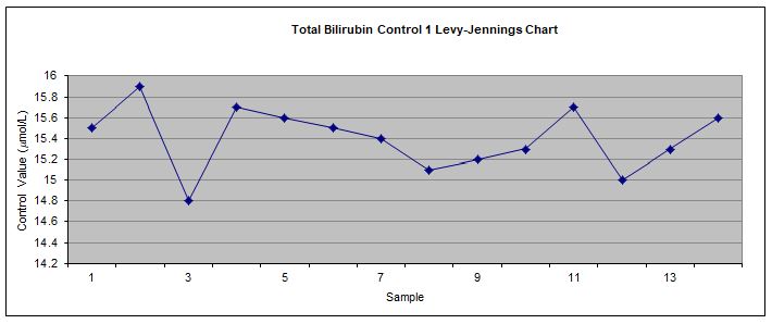
Figure 9 Levy-Jennings chart used to monitor internal QAP for control 1.

 

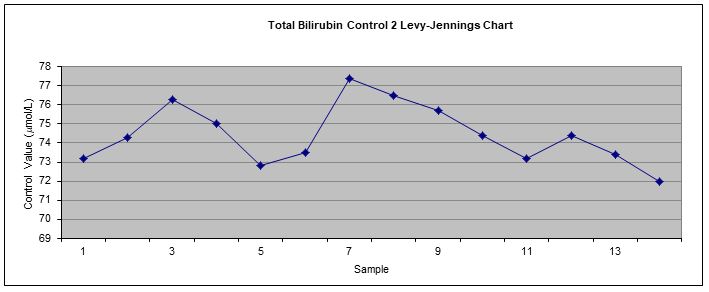
Figure 10 Levy-Jennings chart used to monitor internal QAP for control 2.

 

References:

1. Joseph A, Samant H. Jaundice. StatPearls [Internet]: StatPearls Publishing; 2019.
2. Kalakonda A, John S. Physiology, Bilirubin. 2017.
3. Berg JM, Tymoczko JL, Stryer L. Biochemistry/Jeremy M. Berg, John L. Tymoczko, Lubert Stryer; with Gregory J. Gatto, Jr. New York: WH Freeman; 2012.
4. Berg JMT, T.M. Stryer,L. Biochemistry. 5th ed: W H Freeman; 2002 2002.
5. Burtis CAaB, D.E. Tietz Fundamentals of Clinical Chemistry and Molecular Diagnostics. 7th ed. Sawyer BG, editor. Missouri: Elsevier Saunders; 2015.

 

Are you looking for BILIRUBIN Assay Method Chemistry Assessment Solutions? We are providing Chemistry Assignment Help at a nominal rate with plagiarism free content. Our experienced Best Assignment Writers assist you with all aspects of the subject. Case Study Help is known for quality assignment help in Australia, the UK, the USA and other countries.